Mekanika Orbit: Teknik-Teknik Matematika

"Teknik-Teknik Mekanika dalam IPTEK Antariksa Sangat Perlu Dikembangkan" 

*Arip Nurahman*

Persamaan Kepler

One approach to calculating orbits (mainly used historically) is to use Kepler's equation:

.

where M is the mean anomaly, E is the eccentric anomaly, and is eccentricty.

With Kepler's formula, finding the time-of-flight to reach an angle (true anomaly) of θ from periapsis is broken into two steps:

1. Compute the eccentric anomaly E from true anomaly θ
2. Compute the time-of-flight t from the eccentric anomaly E

Finding the angle at a given time is harder. Kepler's equation is transcendental in E, meaning it cannot be solved for E analytically, and so numerical approaches must be used. In effect, one must guess a value of E and solve for time-of-flight; then adjust E as necessary to bring the computed time-of-flight closer to the desired value until the required precision is achieved. Usually, Newton's method is used to achieve relatively fast convergence.

The main difficulty with this approach is that it can take prohibitively long to converge for the extreme elliptical orbits. For near-parabolic orbits, eccentricity e is nearly 1, and plugging e = 1 into the formula for mean anomaly, E − sinE, we find ourselves subtracting two nearly-equal values, and so accuracy suffers. For near-circular orbits, it is hard to find the periapsis in the first place (and truly circular orbits have no periapsis at all). Furthermore, the equation was derived on the assumption of an elliptical orbit, and so it does not hold for parabolic or hyperbolic orbits at all. These difficulties are what led to the development of the universal variable formulation, described below.

Perturbation theory

Main article: Perturbation theory

One can deal with perturbations just by summing the forces and integrating, but that is not always best. Historically, variation of parameters has been used which is easier to mathematically apply with when perturbations are small.

Conic orbits

For simple procedures, such as computing the delta-v for coplanar transfer ellipses, traditional approaches^{[clarification needed]} are fairly effective. Others, such as time-of-flight are far more complicated, especially for near-circular and hyperbolic orbits.

The patched conic approximation

The transfer orbit alone is a poor approximation for interplanetary trajectories because it neglects the planets' own gravity. Planetary gravity dominates the behaviour of the spacecraft in the vicinity of a planet. It severely underestimates delta-v, and produces highly inaccurate prescriptions for burn timings.

A relatively simple way to get a first-order approximation of delta-v is based on the patched conic approximation technique. One must choose the one dominant gravitating body in each region of space through which the trajectory will pass, and to model only that body's effects in that region. For instance, on a trajectory from the Earth to Mars, one would begin by considering only the Earth's gravity until the trajectory reaches a distance where the Earth's gravity no longer dominates that of the Sun.

The spacecraft would be given escape velocity to send it on its way to interplanetary space. Next, one would consider only the Sun's gravity until the trajectory reaches the neighbourhood of Mars. During this stage, the transfer orbit model is appropriate. Finally, only Mars's gravity is considered during the final portion of the trajectory where Mars's gravity dominates the spacecraft's behaviour.

The spacecraft would approach Mars on a hyperbolic orbit, and a final retrograde burn would slow the spacecraft enough to be captured by Mars.

The size of the "neighborhoods" (or spheres of influence) vary with radius r_SOI:

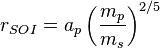
where a_p is the semimajor axis of the planet's orbit relative to the Sun; m_p and m_s are the masses of the planet and Sun, respectively.

This simplification is sufficient to compute rough estimates of fuel requirements, and rough time-of-flight estimates, but it is not generally accurate enough to guide a spacecraft to its destination. For that, numerical methods are required.

The universal variable formulation

To address the shortcomings of the traditional approaches, the universal variable formulation was developed. It works equally well on circular, elliptical, parabolic, and hyperbolic orbits; and also works well with perturbation theory. The differential equations converge nicely when integrated for any orbit.

Perturbations

The universal variable formulation works well with the variation of parameters technique, except now, instead of the six Keplerian orbital elements, we use a different set of orbital elements: namely, the satellite's initial position and velocity vectors x₀ and v₀ at a given epoch t = 0.

In a two-body simulation, these elements are sufficient to compute the satellite's position and velocity at any time in the future, using the universal variable formulation.

Conversely, at any moment in the satellite's orbit, we can measure its position and velocity, and then use the universal variable approach to determine what its initial position and velocity would have been at the epoch. In perfect two-body motion, these orbital elements would be invariant (just like the Keplerian elements would be).

However, perturbations cause the orbital elements to change over time. Hence, we write the position element as x₀(t) and the velocity element as v₀(t), indicating that they vary with time. The technique to compute the effect of perturbations becomes one of finding expressions, either exact or approximate, for the functions x₀(t) and v₀(t).

Non-ideal orbits

The following are some effects which make real orbits differ from the simple models based on a spherical earth. Most of them can be handled on short timescales (perhaps less than a few thousand orbits) by perturbation theory because they are small relative to the corresponding two-body effects.

• Equatorial bulges cause precession of the node and the perigee
• Tesseral harmonics of the gravity field introduce additional perturbations
• lunar and solar gravity perturbations alter the orbits
• Atmospheric drag reduces the semi-major axis unless make-up thrust is used

Over very long timescales (perhaps millions of orbits), even small perturbations can dominate, and the behaviour can become chaotic.

On the other hand, the various perturbations can be orchestrated by clever astrodynamicists to assist with orbit maintenance tasks, such as station-keeping, ground track maintenance or adjustment, or phasing of perigee to cover selected targets at low altitude.

Sumber:

Wikipedia